American Express - Default Prediction
Built a classification model to predict the probability that a customer does not pay back their credit card balance (defaults) based on their monthly customer statements using the data provided by American Express.

-
Built a classification model to predict the probability that a customer does not pay back their credit card balance (defaults) based on their monthly customer statements using the data provided by American Express.
-
The data was particularly challenging to deal with as it had 5.5 million records and 191 anonymized features. 122 features had more than 10% missing values. The target variable had severe class imbalance.
-
Engineered new features by taking different aggregations over time which helped increase model accuracy by 12%.
-
Optimized XGBoost and LightGBM Classifiers using RandomSearchCV to reach the best model.
-
A Soft-Voting Ensemble of the best performing XGBoost and LightGBM Models was used to make final predictions which yielded an Accuracy of 94.48%, an F1-Score of 96.71% and an ROC-AUC Score of 96.40%.
Data
Credit default prediction is central to managing risk in a consumer lending business. Credit default prediction allows lenders to optimize lending decisions, which leads to a better customer experience and sound business economics.
The dataset contains profile features for each customer at each statement date. Features are anonymized and normalized, and fall into the following general categories:
D_* = Delinquency variables
S_* = Spend variables
P_* = Payment variables
B_* = Balance variables
R_* = Risk variables
with the following features being categorical:
'B_30', 'B_38', 'D_114', 'D_116', 'D_117', 'D_120', 'D_126', 'D_63', 'D_64', 'D_66', 'D_68'
The dataset can be downloaded from here.
Analysis
The complete analysis can be viewed here.
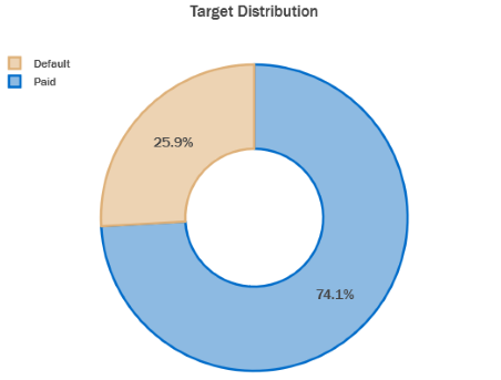
Target Distribution
- In the data present we observe that 25.9% of records have defaulted on their credit card payments whereas 74.1% have paid their bills on time.
- This distribution shows us that there is severe class imbalance present.
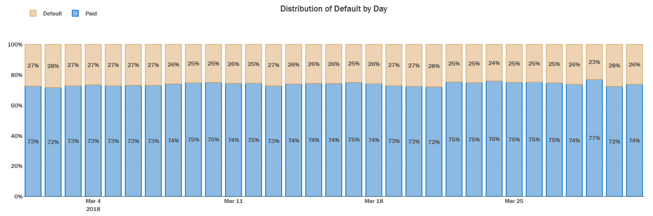
Distribution of Number of Defaults per day for the first Month:
The proportion of customers that defualt is consistent across each day in the data, with a slight weekly seasonal trend influenced by the day when the customers receive their statements.
Frequency of Customer Statements for the first month:
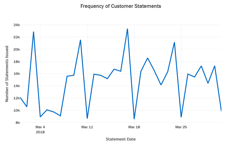
- There is weekly seasonal pattern observed in the number of statements received per day.
- As seen above this trend does not seem to be significantly affecting the proportion of default.
Distribution of values of Payment Variables:
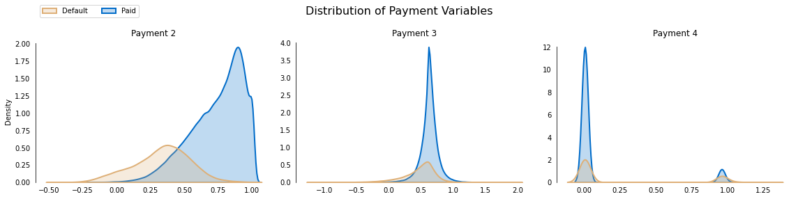
- We notice that Payment 2 is heavily negatively skewed (left skewed).
- Even though Payment 4 have continuous values between 0 and 1, most of the density is clustered around 0 and 1.
- This tells us that there may be some Gaussian Noise present. The noise can be removed and into a binary variable.
Correlation of Features with Target Variable:
- Payment 2 is negatively correlated with the target with a correlation of -0.67.
- Delinquency 48 is positively correlated with the target with a correlation of 0.61.
Correlation of Payment Variables with Target
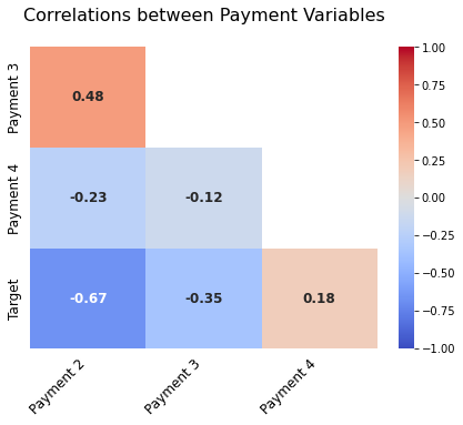
- We observe that Payment 2 and Target are highly negatively correlated.
- This could be probably be due to the fact that people paying their bill have a less chance of default.
Experiments:
-
The dataset presents a significant challenge with a substantial number of missing values, making imputation impossible due to the anonymization of features and the lack of a clear rationale behind imputation. This unique constraint compels us to select models that are capable of handling missing values, pushing us to explore advanced techniques.
-
One notable characteristic of the dataset is its high cardinality, boasting an impressive 191 features. However, the presence of missing values poses limitations on the utilization of conventional dimensionality reduction techniques like Principal Component Analysis (PCA) and feature selection methods such as Recursive Feature Elimination (RFE). Thus, we must seek alternative approaches to tackle this challenge.
-
In order to overcome the limitations imposed by missing values, we employ a creative strategy: engineering new features through aggregations over the time dimension. By disregarding missing values during the aggregation process, we generate dense and informative engineered features that can be effectively utilized for modeling purposes.
-
Several prominent classification models that gracefully handle missing values have been considered for this task, including XGBoost, LightGBM, and CatBoost. Notably, these models internally incorporate imputation techniques, dynamically adapting them based on the approach that yields the greatest performance improvement. This ensures that missing values do not impede the model's ability to make accurate predictions.
-
To establish a performance baseline, an XGBoost model with default hyperparameters was trained, yielding an impressive accuracy of 78.84%, an F1-Score of 54.64%, and an ROC-AUC Score of 65.72%. These results serve as a solid starting point for further improvement.
-
Subsequently, the LightGBM model with default hyperparameters was employed, resulting in notable enhancements across performance metrics. Specifically, the LightGBM model boosted the accuracy by 1%, the F1-Score by 12%, and the ROC-AUC Score by 6%, further solidifying its effectiveness.
-
To fine-tune the XGBoost and LightGBM models, a Randomized Grid Search was conducted utilizing 5-fold cross-validation. This comprehensive search approach allowed us to explore a wide range of hyperparameter combinations efficiently.
-
Hyperparameters of the XGBoost model, such as
n_estimators,max_depth, andlearning_rate, were meticulously tuned, resulting in remarkable improvements. The accuracy was enhanced by 9%, the F1-Score by 18%, and the ROC-AUC Score by 3%, showcasing the model's capacity to capture more nuanced patterns in the data. -
Similarly, the hyperparameters of the LightGBM model, including
n_estimators,feature_fraction, andlearning_rate, were fine-tuned through the Randomized Grid Search. This meticulous optimization process led to a marginal but meaningful accuracy improvement of 0.1%, an F1-Score boost of 6%, and an impressive 10% enhancement in the ROC-AUC Score.
By utilizing advanced techniques, engineering informative features, and fine-tuning the models through extensive hyperparameter optimization, we were able to elevate the performance of both the XGBoost and LightGBM models while gracefully handling the challenges imposed by missing values and high feature cardinality.
Results:
A Soft Voting Classifier was used to create a ensemble of both the models and was used for generating the final predictions. It achieved an Accuracy of 94.48%, an F1-Score of 96.71% and an ROC-AUC Score of 96.40%.
The results from all the models have been summarized below:
| Model | Accuracy | F1-Score | ROC-AUC Score |
|---|---|---|---|
| XGBoost (default) | 78.84 | 54.64 | 65.72 |
| LightGBM (default) | 79.84 | 62.92 | 71.86 |
| XGBoost (fine-tuned) | 88.61 | 80.74 | 74.96 |
| LightGBM (fine-tuned) | 88.72 | 86.42 | 84.22 |
| Voting Classifier (XGB + LGBM) | 94.48 | 96.72 | 96.40 |
Run Locally
The code to run the project can be found here: American Express - Default Prediction Github.
- Install required libraries:
pip install -r requirements.txt
- Generate features:
python amex-feature-engg.py
- Fine-tune models:
python amex-fine-tuning.py
- Generate predictions:
python amex-final-prediction.py
Feedback
If you have any feedback, please reach out to me.